This post keep track of what I realized and learned through building GAP. Reason: No mobile printing service at gatech, only mac and windows officially supported, (I guess the reason is they think people using linux can figure it out themselves).

I googled for the info, one I can think of for now is setup the server on android and add printers to the server, and use terminal with busybox tool set (just lpr i guess) to print like on linux. But this comes with a lot of barriers and of course is not the best way to do it.However, For now I should focus on how to make it run first. I should embed busybox into the printing app and make an user interface for the command input later.Also I should make and implicit intent for other apps to launch printing. Later if time allowed, I could do a auto connect to gatech network though their vpn for my user if they are not using gatech internet. (gatech only allows sending print request from inland network). My approach: starting from a open source built CUPS services app. Since there is a server provided by this app through advanced setting. I could configure it with the gatech printer configuration.

Here is a summary for the recent work I’ve done with my colleague at GTRI. The work is based on the work in papers section.The basic idea is let computer categorize the scenes given a short time of video, say 20 secs.What we did is actually transforming the research results into real time application. You can find a demo at here. It’s still pretty primitive if you see outfit we have to wear for this. The most important part is we have to use fast cpu and GPU to run through caffe to get the outputMaps for the frames we capture and then calculate the fisher vector for the current segments(20 secs video) and calculate the distance between the fisher vector for the current segments and fisher vectors we have in our database in real time. To this end, other wearable devices can’t get the job done because the limitation of the their GPU and compatibility issue with caffe.

I’ve seen someone port caffe on android devices on Github using JNI, but it’s running on CPU. I’ve tried one of it’s application to classify to objects from Nexus 6’s camera, it took around 10 secs to finish the whole process given it’s not optimized code. It’s not bad but I have to admit the hardware is still a drawback for deep learning application to run on mobile devices. Maybe currently we have to depend on uploading videos to servers to process but that gonna take a lot of time transferring data plus it’s not friendly to people with limited data plan.

I still remember the hardest time when me and Robert sitting together debugging the caffe code for this project, it was like not making progress at all.But finally we persisted and came through all the problems thanks to our great collaboration and communication as well as helps from Dr.Wagner and Dr.Kira. I feels I’ve learned a lot from this working experience: getting better understanding in coding in c/c++ and python, working collaboratively using Git and Github, setting up hardware within our project and of course how to use adobe premiere to edit videos…I feels like working in a group is pretty great, I can learn from different people, talk to them, asking questions when get confused.

Below are simplified docs for this project(it’s a private repo,can’t share to much here):

#Hardwares

• Point Grey Research Grasshopper3 camera
• Google Glass for training data
  • relative aperture: f/2.48
  • focal length: 2.95mm
  • Videos - 720p

#Dependencies

Flycapture2-SDK
Opencv-2.4.8
boost-1.54.0.1ubuntu1
caffe
ffmpeg-2.62
vlfeat-0.9.20
cmake/eclipse with cdt

#Usage

Preprocess

• Videos to Images:Just a python script using ffmpeg to convert videos to frames

DeepsegmentsApp

• Training the Gaussian Mixture Model (classifying outputMaps from frames).
• Running the classifying application with auditory output for users.

FeatureExtractionApp

Application for extracting features based on output maps of convolutional neural network.

• Sequential extraction: for this to run, we assume you have a root folder for all the video frames and each video has frames under its own folder(example: root_video_frames/zoo/1.jpg). We currently save outputMaps to binary to save storage.
• Testing output for fc8 layer: we support sending an image to CNN with a prediction as output.
• During sequential extraction you can stop the process anytime, just run the same command, it will restart from where it was left to folder level.
• This app assume working directory /home/user/projects/caffe and /home/user/projects/DeepSegments.

#Papers

Doshi, J., Mason, C., Wagner, A.R., Kira, Z., “Deep Segments: Comparisons between Scenes and their Constituent Fragments using Deep Learning”. Georgia Tech technical report, GT-CS-14-07, 2014. pdf

Doshi, J., Kira, Z., and Wagner, A.R., “From Deep Learning to Episodic Memories: Creating Categories of Visual Experiences”, accepted to the Third Annual Conference on Advances in Cognitive Systems (ACS), 2015.pdf

It’s been a while, I complete this competition with my friend and we rank top 25% for the first time we participate in kaggle machine learning competition. I have to say I learned and realized a lot through this competition. I learned a lot more tools to build machine learning system as well as which are best for what, say, scikit learn lib still using sequential algorithm with made it pretty slow to get the feedback although it is the most resourceful machine learning library in python to test for ideas, several other python libs like keras and lasagne is good for using gpu through theano to run neural networks. I realized neural network is not the only best tool to use for machine learning, but ensemble skills are, (bagging and boosting, etc). Neural network is only one expert that ensemble built upon for this prediction.

Here I copy the winner’s solution to remind me I still a newbie. 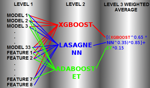Our solution is based in a 3-layer learning architecture as shown in the picture attached. -1st level: there are about 33 models that we used their predictions as meta features for the 2nd level, also there are 8 engineered features. -2nd level: there are 3 models trained using 33 meta features + 7 features from 1st level: XGBOOST, Neural Network(NN) and ADABOOST with ExtraTrees. -3rd level: it’s composed by a weighted mean of 2nd level predictions. All models in 1st layers are trained using a 5 fold cross-validation technique using always the same fold indices.

The 2nd level we trainned using 4 Kfold random indices. It provided us the ability to calculate the score before submitting to the leader board. All our cross-validate scores are extremely correlated with LB scores, so we have a good estimate of performance locally and it enabled us the ability to discard useless models for the 2nd learning level.

Models and features used for 2nd level training:

X = Train and test sets

-Model 1: RandomForest(R). Dataset: X -Model 2: Logistic Regression(scikit). Dataset: Log(X+1) -Model 3: Extra Trees Classifier(scikit). Dataset: Log(X+1) (but could be raw) -Model 4: KNeighborsClassifier(scikit). Dataset: Scale( Log(X+1) ) -Model 5: libfm. Dataset: Sparse(X). Each feature value is a unique level. -Model 6: H2O NN. Bag of 10 runs. Dataset: sqrt( X + 3/8) -Model 7: Multinomial Naive Bayes(scikit). Dataset: Log(X+1) -Model 8: Lasagne NN(CPU). Bag of 2 NN runs. First with Dataset Scale( Log(X+1) ) and second with Dataset Scale( X ) -Model 9: Lasagne NN(CPU). Bag of 6 runs. Dataset: Scale( Log(X+1) ) -Model 10: T-sne. Dimension reduction to 3 dimensions. Also stacked 2 kmeans features using the T-sne 3 dimensions. Dataset: Log(X+1) -Model 11: Sofia(R). Dataset: one against all with learner_type=”logreg-pegasos” and loop_type=”balanced-stochastic”. Dataset: Scale(X) -Model 12: Sofia(R). Trainned one against all with learner_type=”logreg-pegasos” and loop_type=”balanced-stochastic”. Dataset: Scale(X, T-sne Dimension, some 3 level interactions between 13 most important features based in randomForest importance ) -Model 13: Sofia(R). Trainned one against all with learner_type=”logreg-pegasos” and loop_type=”combined-roc”. Dataset: Log(1+X, T-sne Dimension, some 3 level interactions between 13 most important features based in randomForest importance ) -Model 14: Xgboost(R). Trainned one against all. Dataset: (X, feature sum(zeros) by row ). Replaced zeros with NA. -Model 15: Xgboost(R). Trainned Multiclass Soft-Prob. Dataset: (X, 7 Kmeans features with different number of clusters, rowSums(X==0), rowSums(Scale(X)>0.5), rowSums(Scale(X)< -0.5) ) -Model 16: Xgboost(R). Trainned Multiclass Soft-Prob. Dataset: (X, T-sne features, Some Kmeans clusters of X) -Model 17: Xgboost(R): Trainned Multiclass Soft-Prob. Dataset: (X, T-sne features, Some Kmeans clusters of log(1+X) ) -Model 18: Xgboost(R): Trainned Multiclass Soft-Prob. Dataset: (X, T-sne features, Some Kmeans clusters of Scale(X) ) -Model 19: Lasagne NN(GPU). 2-Layer. Bag of 120 NN runs with different number of epochs. -Model 20: Lasagne NN(GPU). 3-Layer. Bag of 120 NN runs with different number of epochs. -Model 21: XGboost. Trained on raw features. Extremely bagged (30 times averaged). -Model 22: KNN on features X + int(X == 0) -Model 23: KNN on features X + int(X == 0) + log(X + 1) -Model 24: KNN on raw with 2 neighbours -Model 25: KNN on raw with 4 neighbours -Model 26: KNN on raw with 8 neighbours -Model 27: KNN on raw with 16 neighbours -Model 28: KNN on raw with 32 neighbours -Model 29: KNN on raw with 64 neighbours -Model 30: KNN on raw with 128 neighbours -Model 31: KNN on raw with 256 neighbours -Model 32: KNN on raw with 512 neighbours -Model 33: KNN on raw with 1024 neighbours -Feature 1: Distances to nearest neighbours of each classes -Feature 2: Sum of distances of 2 nearest neighbours of each classes -Feature 3: Sum of distances of 4 nearest neighbours of each classes -Feature 4: Distances to nearest neighbours of each classes in TFIDF space -Feature 5: Distances to nearest neighbours of each classed in T-SNE space (3 dimensions) -Feature 6: Clustering features of original dataset -Feature 7: Number of non-zeros elements in each row -Feature 8: X (That feature was used only in NN 2nd level training)

The 2nd level we start training cross-validated just to choose best models, tune hyperparameters and find optimum weights to average 3rd level. After we found some good parameters, we trained 2nd level using entire trainset and bagged results. The final model is a very stable 2nd level bagging of: XGBOOST: 250 runs. NN: 600 runs. ADABOOST: 250 runs.

The average for the 3rd level we found better using a geometric mean of XGBOOST and NN. For ET we did an aritmetic mean with previous result: 0.85 * [XGBOOST^0.65 * NN^0.35] + 0.15 * [ET].

We tried a lot of training algorithms in first level as Vowpal Wabbit(many configurations), R glm, glmnet, scikit SVC, SVR, Ridge, SGD, etc… but none of these helped improving performance on second level. Also we tried some preprocessing like PCA, ICA and FFT without improvement. Also we tried Feature Selection without improvement. It seems that all features have positive prediction power. Also we tried semi-supervised learning without relevant improvement and we discarded it due the fact that it have great potential to overfit our results.

Definetely the best algorithms to solve this problem are: Xgboost, NN and KNN. T-sne reduction also helped a lot. Other algorithm have a minor participation on performance. So we learn not to discard low performance algorithms, since it have enough predictive power to improve performance in a 2nd level training. Our final cross-validated solution scored around 0.3962. LB(Public): 0.38055 and LB(Private): 0.38243.